# init repo notebook
!git clone https://github.com/rramosp/ppdl.git > /dev/null 2> /dev/null
!mv -n ppdl/content/init.py ppdl/content/local . 2> /dev/null
!pip install -r ppdl/content/requirements.txt > /dev/null

Distribution Lambda

import numpy as np
import matplotlib.pyplot as plt
from scipy import stats
from scipy.integrate import quad
from progressbar import progressbar as pbar
from rlxutils import subplots, copy_func

import tensorflow as tf
import tensorflow_probability as tfp
tfd = tfp.distributions
tfb = tfp.bijectors

%matplotlib inline

2022-02-20 07:56:50.326703: W tensorflow/stream_executor/platform/default/dso_loader.cc:64] Could not load dynamic library 'libcudart.so.11.0'; dlerror: libcudart.so.11.0: cannot open shared object file: No such file or directory
2022-02-20 07:56:50.326739: I tensorflow/stream_executor/cuda/cudart_stub.cc:29] Ignore above cudart dlerror if you do not have a GPU set up on your machine.

import os
os.environ["CUDA_VISIBLE_DEVICES"] = "-1"

Using distribution objects in Keras models

TFP provides several layer objects so that we can include distributions in Keras models. This is useful because this would allow us to learn distribution parameters with the regular model machinery of Keras, such as using Dense layers, transforming data, etc.

tfp.layers.VariableLayer

Simply produces a constant value that can be trainable. It is equivalent to a Dense Keras layer with the kernel set to zero and only the bias trainable. The output is the same (constant) for any input of any size. It is used to provide values to posterior layers which do not depend on input data (such as paratemeters of distributions).

vl = tfp.layers.VariableLayer(shape=(3,2))
vl

<tensorflow_probability.python.layers.variable_input.VariableLayer at 0x7fe472f814c0>

x = np.random.random(size=(10,4))
vl(x)

<tf.Tensor: shape=(3, 2), dtype=float32, numpy=
array([[0., 0.],
       [0., 0.],
       [0., 0.]], dtype=float32)>

the initializer defines the initial constant value. See tf.keras.initializers and tfp.layers.BlockwiseInitializer

vl = tfp.layers.VariableLayer(shape=(3,2), initializer="ones")
vl(x)

<tf.Tensor: shape=(3, 2), dtype=float32, numpy=
array([[1., 1.],
       [1., 1.],
       [1., 1.]], dtype=float32)>

vl = tfp.layers.VariableLayer(
            shape=(3,2), 
            initializer=tf.keras.initializers.RandomNormal(mean=0., stddev=1.)
     )

vl(x)

<tf.Tensor: shape=(3, 2), dtype=float32, numpy=
array([[-1.3975693,  1.2439306],
       [-1.4463489, -1.8343785],
       [ 1.1516911, -0.4883429]], dtype=float32)>

the BlockwiseInitializer concatenates other initializers and dimensions must be broadcastable

vl = tfp.layers.VariableLayer(shape=(3,2), initializer=
    tfp.layers.BlockwiseInitializer([
          'zeros',
           tf.keras.initializers.Constant(np.log(np.expm1(1.))),  # = 0.541325
        ], 
        sizes=[1, 1])
    )

vl(x)

<tf.Tensor: shape=(3, 2), dtype=float32, numpy=
array([[0.        , 0.54132485],
       [0.        , 0.54132485],
       [0.        , 0.54132485]], dtype=float32)>

tfp.layers.DistributionLambda

They provide a wrapper for tfp distribution objects so that they can be integrated in Keras models. Observe that their parameter is a function, so that it can be invoked by Keras within a GradientTape.

We can choose to use variables for distribution the distribution parameters, and use the input data ONLY to evaluate the loss.

Observe we use a VariableLayer to create a variable in the middle of the model

x = 5*tfd.Beta(2.,5).sample(10000)+2

inp = tf.keras.layers.Input(shape=(1,))
var = tfp.layers.VariableLayer(shape=(2), initializer="ones")(inp)
out = tfp.layers.DistributionLambda(lambda t: tfd.Normal(loc=t[0], scale=tf.math.softplus(t[1])))(var)

m   = tf.keras.models.Model(inp, out)

2022-02-20 07:57:04.730721: W tensorflow/python/util/util.cc:368] Sets are not currently considered sequences, but this may change in the future, so consider avoiding using them.

m.weights

[<tf.Variable 'constant:0' shape=(2,) dtype=float32, numpy=array([1., 1.], dtype=float32)>]

we get always the same distribution regardless the input, in this case with mean and softplus std as initialized in the VariableLayer.

_x = m([np.random.random()]).sample(100000).numpy()
_x.mean(), _x.std(), tf.math.softplus(1.).numpy()

(1.0002679, 1.3119836, 1.3132616)

the loss function takes the target and the model output. NOTICE that the model output is a distribution object, so we can use its methods.

negloglik = lambda x, distribution: -distribution.log_prob(x)
m.compile(optimizer='adam', loss=negloglik)

negloglik(x, tfd.Normal(0,1))

<tf.Tensor: shape=(10000,), dtype=float32, numpy=
array([4.533191 , 5.8602905, 8.682795 , ..., 5.0683117, 6.6048856,
       4.1267476], dtype=float32)>

the model does not use the input, we only to provide the target to the .fit so that it can pass it on to the loss function.

dummy_input = np.random.random(len(x))
m.fit(dummy_input, x, epochs=40, verbose=0)

<keras.callbacks.History at 0x7fe472d58af0>

# the weights are in the variables of the VariableLayer
m.weights

[<tf.Variable 'constant:0' shape=(2,) dtype=float32, numpy=array([3.4179287 , 0.20450164], dtype=float32)>]

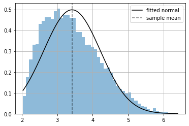
This is a very particular setting, since the output DOES NOT depend on the input, it is just a distribution whose parameters have been previously learnt. The target is only used in the loss function. Once training is complete the loss function is not needed anymore.

distribution = m([np.random.random()])

xr = np.linspace(np.min(x), np.max(x), 100)
plt.hist(x.numpy(), bins=50, density=True, alpha=.5);
plt.plot(xr, np.exp(distribution.log_prob(xr).numpy()), color="black", label="fitted normal");
plt.axvline(np.mean(x), ls="--", color="black", alpha=.5, label="sample mean")
plt.grid(); plt.legend();

Learning a distribution for each input data point

The setting above seems a bit unnatural for Keras. In fact, the full power of TFP unveils when we learn a distribution for each input data point.

More in depth observe that:

• The output of the layer when using the implicit call method of the layer is a distribution.

• The output of the layer when using the predict method of a model is a sample from the distribution.

• It can use the output of previous layers as parameters for the distribution

For comparison consider a model with a regular keras model, where call and predict have the same behaviour.

inp  = tf.keras.layers.Input(shape=(1,))
out  = tf.keras.layers.Dense(2)(inp)
m    = tf.keras.models.Model(inp, out)

x = np.r_[1.,2.,3.].reshape(-1,1)

# using the implicit call method of the model
m(x)

<tf.Tensor: shape=(3, 2), dtype=float32, numpy=
array([[-1.0067325,  1.0000728],
       [-2.013465 ,  2.0001457],
       [-3.0201974,  3.0002184]], dtype=float32)>

# using the implicit call method of the layer
m.layers[1](x)

<tf.Tensor: shape=(3, 2), dtype=float32, numpy=
array([[-1.0067325,  1.0000728],
       [-2.013465 ,  2.0001457],
       [-3.0201974,  3.0002184]], dtype=float32)>

# using the predict method of the model
m.predict(x)

array([[-1.0067325,  1.0000728],
       [-2.013465 ,  2.0001457],
       [-3.0201974,  3.0002184]], dtype=float32)

Now with a DistributionLambda layer. Observe that we choose to use the output of the previous layer to be the mean (first column) and std (second column) of the distribution

inp = tf.keras.layers.Input(shape=(2,))
out = tfp.layers.DistributionLambda(lambda t: tfd.Normal(loc=t[:,0], scale=t[:,1]))(inp)

m   = tf.keras.models.Model(inp, out)

x = np.r_[1.,2.,10.,4.,20.,6.].reshape(3,2)
x

array([[ 1.,  2.],
       [10.,  4.],
       [20.,  6.]])

we implicitly use the call method of our model. Observe we get one distribution for each input data, which shows up in the batch_size.

m(x)

<tfp.distributions._TensorCoercible 'tensor_coercible' batch_shape=[3] event_shape=[] dtype=float32>

which is the same as if we call directly the DistributionLambda layer object.

m.layers[1](x)

<tfp.distributions._TensorCoercible 'tensor_coercible' batch_shape=[3] event_shape=[] dtype=float32>

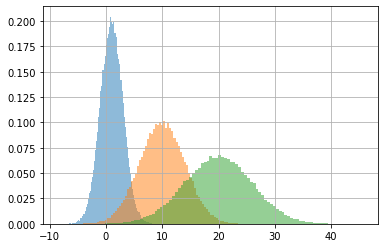
we can sample this output distribution. Each sample will contain three elements, one per data point following a normal distribution parametrized by the two elements of the data point (mean and std).

_x = m(x).sample(100000).numpy()
_x.shape

(100000, 3)

_x.mean(axis=0), _x.std(axis=0)

(array([ 1.004689,  9.983776, 19.96568 ], dtype=float32),
 array([2.003365 , 3.9917862, 5.986713 ], dtype=float32))

for i in range(len(x)):
    plt.hist(_x[:,i], density=True, bins=100, alpha=.5)
plt.grid();

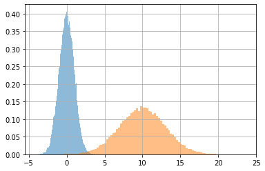
In this case, the .predict method behaves differently from the implicit call. It produces a sample following the input data.

This behaviour can be changed by the convert_to_tensor_fn argument. See the DistributionLambda docs. So that you could return the distribution mean, or any other representative value you want to have as a result of a predictions. Sampling from the distribution corresponding to each input data point is a generally convenient choice for generative models.

# the predictions (samples) follow the distributions parametrized by x
x = np.concatenate([np.r_[[[0,1]]*40000], np.r_[[[10,3]]*50000]])
x.shape

(90000, 2)

_x = m.predict(x)
_x.shape

(90000,)

_x[:40000].mean(), _x[:40000].std(), "::", _x[40000:].mean(), _x[40000:].std()

(-0.0049270834, 1.0014801, '::', 9.986944, 3.0177207)

plt.hist(_x[:40000], alpha=.5, density=True, bins=100)
plt.hist(_x[40000:], alpha=.5, density=True, bins=100);
plt.grid();

Learning distribution parameters

We have not fit any model yet, but we can use this machinery to learn the distribution parameters for each input data point with a small Dense layer.

We are trying to learn this model

\[\begin{split} \begin{align} \mu_x, \sigma_x &= D_\theta(x) \\ y &\sim \mathcal{N}(\mu_x, \sigma_x) \end{align} \end{split}\]

where \(D_\theta\) is a regular neural network with parameters \(\theta\) which, given an input \(x\), returns two values \(\mu_x\) and \(\sigma_x\). These two values will be used to parametrize a gaussian distribution for that specific \(x\).

and we want \(\theta\) that maximizes the log likelihood.

\[\underset{\theta}{\text{arg min}}\;\; - \frac{1}{N} \sum_{x_i} \log P_{\mathcal{N}(\mu_{x_i}, \sigma_{x_i})}(x_i)\]

Observe that, this way, we have a predictive distribution for each input data point.

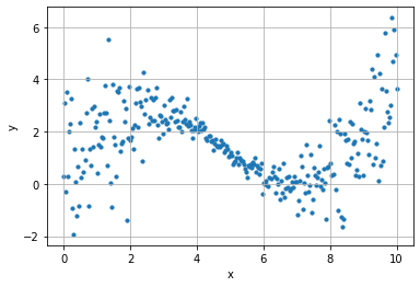
n_points = 300
k = 2
x = np.linspace(0, 10, n_points)
y = .3*x+2*np.sin(x/1.5) + (.2+.02* ((x-5)*k)**2) * np.random.randn(n_points)

plt.scatter(x, y, s=10)
plt.grid();
plt.xlabel("x"); plt.ylabel("y")

Text(0, 0.5, 'y')

inp  = tf.keras.layers.Input(shape=(1,))
out  = tf.keras.layers.Dense(10, activation="tanh")(inp)
out  = tf.keras.layers.Dense(10, activation="tanh")(out)
out  = tf.keras.layers.Dense(2)(out)
out  = tfp.layers.DistributionLambda(lambda t: tfd.Normal(loc=t[:,0], scale=tf.math.softplus(t[:,1])))(out)

m    = tf.keras.models.Model(inp, out)

m.summary()

Model: "model_4"
_________________________________________________________________
 Layer (type)                Output Shape              Param #   
=================================================================
 input_5 (InputLayer)        [(None, 1)]               0         
                                                                 
 dense_2 (Dense)             (None, 10)                20        
                                                                 
 dense_3 (Dense)             (None, 10)                110       
                                                                 
 dense_4 (Dense)             (None, 2)                 22        
                                                                 
 distribution_lambda_2 (Dist  ((None,),                0         
 ributionLambda)              (None,))                           
                                                                 
=================================================================
Total params: 152
Trainable params: 152
Non-trainable params: 0
_________________________________________________________________

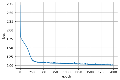
negloglik = lambda x, distribution: -distribution.log_prob(x)
m.compile(optimizer='adam', loss=negloglik)

history = m.fit(x,y, epochs=2000, verbose=0)

plt.plot(history.epoch, history.history['loss'])
plt.grid(); plt.xlabel("epoch"); plt.ylabel("loss");

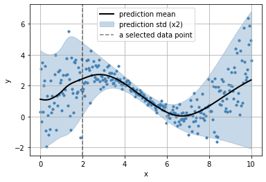
get the predictive distributions for each input data point

_y = m(x)
_y

<tfp.distributions._TensorCoercible 'tensor_coercible' batch_shape=[300] event_shape=[] dtype=float32>

observe the parameters learn for each datapoint

_x = np.r_[2]

plt.scatter(x, y, s=10, color="steelblue")
plt.plot(x, _y.parameters['loc'], color="black", lw=2, label="prediction mean")
plt.fill_between(x, 
                 _y.parameters['loc'] + 2*_y.parameters['scale'], 
                 _y.parameters['loc'] - 2*_y.parameters['scale'], alpha=.3, 
                 color="steelblue",
                 label="prediction std (x2)")
plt.axvline(_x[0], color="black", ls="--", alpha=.5, label="a selected data point")
plt.grid(); plt.legend();
plt.xlabel("x"); plt.ylabel("y")

Text(0, 0.5, 'y')

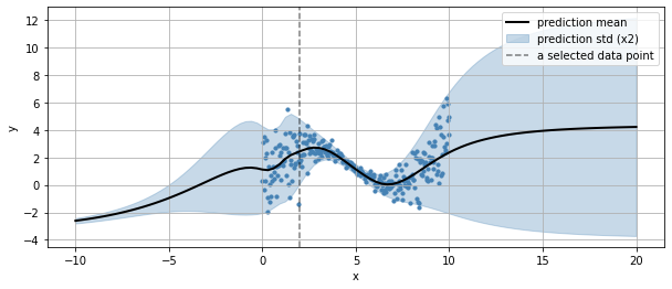
we can also see how it generlizes outside the input variable bounds

xr = np.linspace(np.min(x)-10, np.max(x)+10, 100)
yr = m(xr)

plt.figure(figsize=(10,4))
plt.scatter(x, y, s=10, color="steelblue")
plt.plot(xr, yr.parameters['loc'], color="black", lw=2, label="prediction mean")
plt.fill_between(xr, 
                 yr.parameters['loc'] + 2*yr.parameters['scale'], 
                 yr.parameters['loc'] - 2*yr.parameters['scale'], alpha=.3, 
                 color="steelblue",
                 label="prediction std (x2)")
plt.axvline(_x[0], color="black", ls="--", alpha=.5, label="a selected data point")
plt.grid(); plt.legend();
plt.xlabel("x"); plt.ylabel("y")

Text(0, 0.5, 'y')

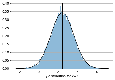
we can get the predictive distribution of any input data point (such as the selected one above)

_xd = m(_x)
_xd

<tfp.distributions._TensorCoercible 'tensor_coercible' batch_shape=[1] event_shape=[] dtype=float32>

_ys = _xd.sample(10000)[:,0].numpy()
_yr = np.linspace(np.min(_ys), np.max(_ys), 100)
plt.plot(_yr, np.exp(_xd.log_prob(_yr)), color="black", alpha=1)
plt.hist(_ys, bins=100, density=True,  alpha=.5);
plt.axvline(_ys.mean(), color="black", lw=3)
plt.grid(); plt.xlabel(f"y distribution for x={_x[0]}")

Text(0.5, 0, 'y distribution for x=2')

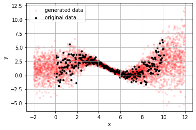
and, since we have distributions we also have a generative model using the .predict method for sampling.

_x = np.random.random(5000)*14-2
_y = m.predict(_x)

plt.scatter(_x, _y, s=10, alpha=.1, color="red",  label="generated data");
plt.scatter(x, y, s=10, alpha=1, color="black", label="original data")
plt.grid(); plt.legend();
plt.xlabel("x"); plt.ylabel("y")

Text(0, 0.5, 'y')